
File:Gradient descent.svg

Size of this PNG preview of this SVG file: 512 × 549 pixels. Other resolutions: 224 × 240 pixels | 448 × 480 pixels | 716 × 768 pixels | 955 × 1,024 pixels | 1,910 × 2,048 pixels.
Original file (SVG file, nominally 512 × 549 pixels, file size: 56 KB)
| This is a file from the Wikimedia Commons. Information from its description page there is shown below. Commons is a freely licensed media file repository. You can help. |
Summary
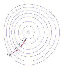
| Description | An illustration of the gradient descent method. I graphed this with Matlab | ||
| Date | (UTC) | ||
| Source |
Own work based on: Gradient descent.png: |
||
| Author |
|
||
| SVG development | This vector image was created with Inkscape. This file uses translateable embedded text.
|
Licensing
I, the copyright holder of this work, hereby publish it under the following license:
| I, the copyright holder of this work, release this work into the public domain. This applies worldwide. In some countries this may not be legally possible; if so: I grant anyone the right to use this work for any purpose, without any conditions, unless such conditions are required by law. |
Source code
% Illustration of gradient descent
function main()

% the ploting window
   figure(1);
   clf; hold on;
   set(gcf, 'color', 'white');
   set(gcf, 'InvertHardCopy', 'off');
   axis equal; axis off;

% the box
   Lx1=-2; Lx2=2; Ly1=-2; Ly2=2;

% the function whose contours will be plotted
   N=60; h=1/N;
   XX=Lx1:h:Lx2;
   YY=Ly1:h:Ly2;
   [X, Y]=meshgrid(XX, YY);
   f=inline('-((y+1).^4/25+(x-1).^4/10+x.^2+y.^2-1)');
   Z=f(X, Y);

% the contours
   h=0.3; l0=-1; l1=20;
   l0=h*floor(l0/h);
   l1=h*floor(l1/h);
   v=[l0:1.5*h:0 0:h:l1 0.8 0.888];
   [c,h] = contour(X, Y, Z, v, 'b');

% graphing settings
   small=0.08;
   small_rad = 0.01;
   thickness=1; arrowsize=0.06; arrow_type=2;
   fontsize=13;
   red = [1, 0, 0];
   white = 0.99*[1, 1, 1];

% initial guess for gradient descent
   x=-0.6498; y=-1.0212;

   % run several iterations of gradient descent
   for i=0:4
      H=text(x-1.5*small, y+small/2, sprintf('x_%d', i));
      set(H, 'fontsize', fontsize, 'color', 0*[1 1 1]);

     % the derivatives in x and in y, the step size
      u=-2/5*(x-1)^3-2*x;
      v=-4/25*(y+1)^3-2*y;
      alpha=0.11;

      if i< 4
         plot([x, x+alpha*u], [y, y+alpha*v]);
         arrow([x, y], [x, y]+alpha*[u, v], thickness, arrowsize, pi/8, ...
               arrow_type, [1, 0, 0])
         x=x+alpha*u; y=y+alpha*v;
      end

   end

% some dummy text, to expand the saving window a bit
   text(-0.9721, -1.5101, '*', 'color', white);
   text(1.5235,   1.1824, '*', 'color', white);

% save to eps
   saveas(gcf, 'Gradient_descent.eps', 'psc2')

function arrow(start, stop, thickness, arrow_size, sharpness, arrow_type, color)

% Function arguments:
% start, stop:  start and end coordinates of arrow, vectors of size 2
% thickness:    thickness of arrow stick
% arrow_size:   the size of the two sides of the angle in this picture ->
% sharpness:    angle between the arrow stick and arrow side, in radians
% arrow_type:   1 for filled arrow, otherwise the arrow will be just two segments
% color:        arrow color, a vector of length three with values in [0, 1]

% convert to complex numbers
   i=sqrt(-1);
   start=start(1)+i*start(2); stop=stop(1)+i*stop(2);
   rotate_angle=exp(i*sharpness);

% points making up the arrow tip (besides the "stop" point)
   point1 = stop - (arrow_size*rotate_angle)*(stop-start)/abs(stop-start);
   point2 = stop - (arrow_size/rotate_angle)*(stop-start)/abs(stop-start);

   if arrow_type==1 % filled arrow

% plot the stick, but not till the end, looks bad
      t=0.5*arrow_size*cos(sharpness)/abs(stop-start); stop1=t*start+(1-t)*stop;
      plot(real([start, stop1]), imag([start, stop1]), 'LineWidth', thickness, 'Color', color);

% fill the arrow
      H=fill(real([stop, point1, point2]), imag([stop, point1, point2]), color);
      set(H, 'EdgeColor', 'none')

   else % two-segment arrow
      plot(real([start, stop]), imag([start, stop]),   'LineWidth', thickness, 'Color', color);
      plot(real([stop, point1]), imag([stop, point1]), 'LineWidth', thickness, 'Color', color);
      plot(real([stop, point2]), imag([stop, point2]), 'LineWidth', thickness, 'Color', color);
   end

function ball(x, y, r, color)
   Theta=0:0.1:2*pi;
   X=r*cos(Theta)+x;
   Y=r*sin(Theta)+y;
   H=fill(X, Y, color);
   set(H, 'EdgeColor', 'none');

%plot2svg must be retrieved from http://www.zhinst.com/blogs/schwizer/
plot2svg;
Original upload log
This image is a derivative work of the following images:
- Gradient descent.png licensed with PD-self
- 2007-06-23T03:33:09Z Oleg Alexandrov 482x529 (25564 Bytes) {{Information |Description=An illustration of the gradient descent method. I graphed this with Matlab |Source=Originally from [http://en.wikipedia.org en.wikipedia]; description page is/was [http://en.wikipedia.org/w/index.ph
Uploaded with derivativeFX
File history
Click on a date/time to view the file as it appeared at that time.
| Date/Time | Thumbnail | Dimensions | User | Comment | |
|---|---|---|---|---|---|
| current | 20:04, 7 August 2012 | | 512 × 549 (56 KB) | wikimediacommons>Zerodamage | == {{int:filedesc}} == {{Information |Description=An illustration of the gradient descent method. I graphed this with Matlab |Source={{Derived from|Gradient_descent.png|display=50}} |Date=2012-08-07 19:02 (UTC) |Author=*File:Gradient_descent.png:... |
File usage
The following page uses this file: